COVID-19's Impact on NYC Traffic Accidents

Introduction

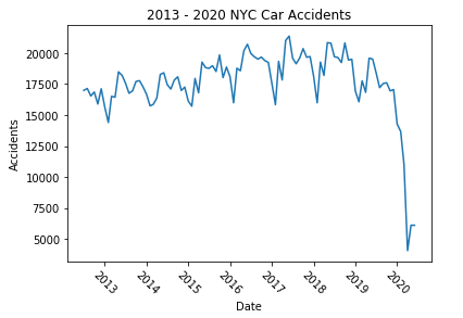
I want to visualize the impact COVID-19 had on monthly NYC traffic accidents. This involved forecasting future months based off previous data not influenced by the pandemic. To complete the time-series forecasting necessary for the analysis I created an ARIMA model. The raw data includes the total number of accidents from 2013 to present-day aggregated by month.

Data Aggregation

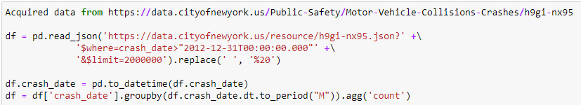
The data was retrieved the NYC Open Data and was in the form of individual accidents. The total number of accidents was much to large (>10m) to import onto my machine, therefore I used the Socrata API to import the sum of accidents by month. The dates I retrieved ranged from January 2013 to June of 2020.

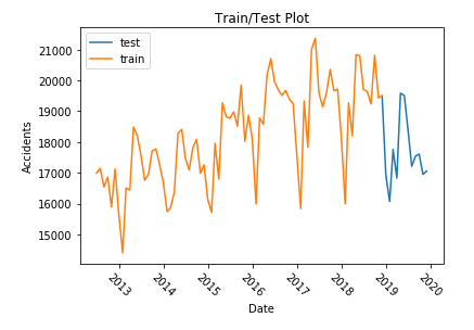
Train/Test

Below is a plot of the NYC Traffic Accidents by month from January 2013 to June 2020

Train: January 2013 - December of 2018.
Test: January 2019 - December 2019.

Stationality

In order to get the data to be stationary the log value was taken and the data was differenced. A plot of the data shows that the rolling mean and rolling standard deviation have low variability. In addition a Dickey-Fuller test was conducted.

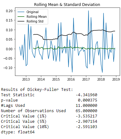
The p-value is less than 0.05 therefor we reject the null-hypothesis and conclude that there is statistical evidence for stationary data. As seen in the graph the rolling mean stays around zero and rolling standard deviation floats around the same value. Now we know for stationality we need to difference the data once, this means our 'd' parameter in our ARIMA model will equal to one.

Optimizing P, D and Q

p: the number of lag observations in the model; also known as the lag order.
d: the number of times that the raw observations are differenced; also known as the degree of differencing.
q: the size of the moving average window; also known as the order of the moving average.
Our ARIMA model requires three parameters and we know our d value is one. Next we use an optimzation algorithm that picks the p and q parameters that have the lowest AIC values.

Modeling

The model now has optimized parameters and was trained using stationary data. We are ready to forecast the next 18 months. The first 12 will be used to analyze how well our model performed, the proceeding six months will be used to analyze effects of COVID-19. Below we see the plot of the 18 month projection.

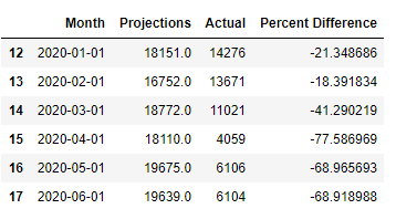
Results

Now we look at a plot of both test data and forecast data ranging from January 2019 through December 2019, in addition to a table of the percent difference between forecasted data and actual data.

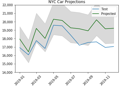
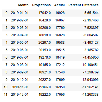
Throughout the year the test set stays within 13% of the projections. Below we see a drastic change in percent difference starting in March. In March accidents were down 41%, by June accidents were reduced by almost 70%.

Github Repository