Predicting pH

Introduction

A soda company is considering hiring a team of data scientests in order to improve the stability and composition of their beverages. Their is a special interest to model and predict pH for quality control and beverage development. A data science team including Layla Quinones, Sergio Ortega, Jack Russo, Neil Shah and myself were given the task to analyse the data and recommend future improvements.

Exploratory Data Analysis

To begin initial insights were gained by acquiring an initial view of the predictors and their corresponding data types.

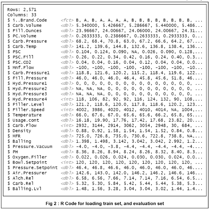
The data revealed 33 columns consisting of 32 predictor variables (31 numerical, one categorical, and the target variable pH. Histograms were created for each variable and can be seen in the github repository at the bottom of this report. The histograms show a variable with little variability as seen below.

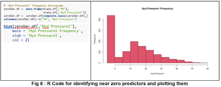
This variable was removed from the data set because many observations had the same value therefore, it does not provide meaningful information about our target variable.

Each column was analyzed for missing values by plotting a histogram and aggregated plot as seen below.

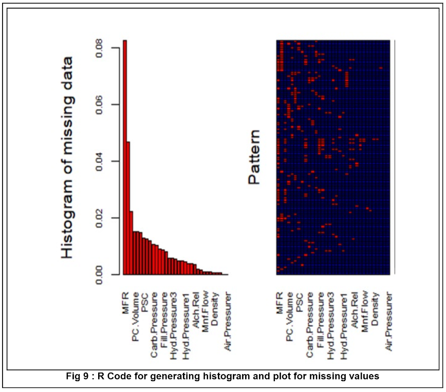
The data had more than 5% of the overall data missing with MFG missing the most values (approximately 8.25%), followed by the categorical variable, Brand Code.

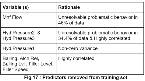
Following the missing data analysis, correlation between predictors is analyzed in order to determine potential multicollinearity or redundancy within the data. The figure below identifies predictor variables that had high correlations.

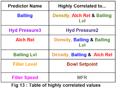
Each highly correlated predictor variable was analyzed in respect to the target variable, pH. Due to correlation Filler Speed, Hyd Pressure2, Hyd Pressure3, and Mnf Flow were removed prior to training our model.

Preprocessing

Prior to imputing data we reduced the complexity of our model through dimensionality reduction for reasons seen below.

After dimensionality reduction the total number of missing values within our data set was 1.2%, a relatively low number for non-categorical predictors. We concluded that random value imputation would minimize cost.

Following imputation we aimed to reduce dimensionality even more through principal component analysis. PCA was applied to all the futures except for our categorical variable. What we found was the the first two principal components (there were 23 total) accounted for about 28% of the variance within the data. The plot below shows PC1 on the x-axis and PC2 on the y-axis.

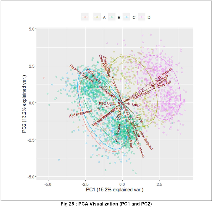
The magnitude and direction of the vector correlates with the contribution towards each principal component. Carb Volume, Carb Pressure, Density, Carb Rel, and Carb Temp all have significant contributions towards PC1. Whereas Carb Pressure, Pressure Vacuum, Carb Flow and Oxygen Filler contribute to most of PC2. The color of each datapoint represents the Brand Code. We see brands D and A have distinguishable characteristics while brands C and B have overlapping components.

Modeling

The datasets were fit to three separate models: multiple linear regression (MLR), random forest and gradient boosting machine. The data was split into an 80/20 training/testing sets. The multiple linear regression was used as a baseline due to simplicity.

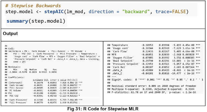
The datasets were fit to three separate models: multiple linear regression (MLR), random forest and gradient boosting machine. The data was split into an 80/20 training/testing sets. The multiple linear regression was used as a baseline due to simplicity, specifically we used a backwards stepwise regression to maximize the adjusted goodness-of-fit.

Next the random forest model was created using 100, 500 and 700 iterations. Increasing the number of iterations is most likely going to have the best performance however it may take too much time depending on the context or require too much processing.

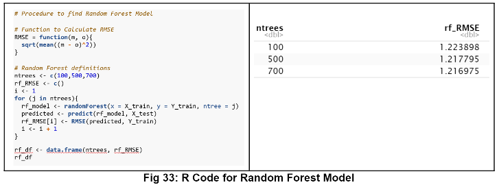
As expected the model using 700 iterations had the lowest RMSE and not extremely long processing time.

The gradient boosted tree model was implemented through the XgBoost library. This model is expected to perform well in respect to random-forest and MLR however it is also expected to have long processing time.

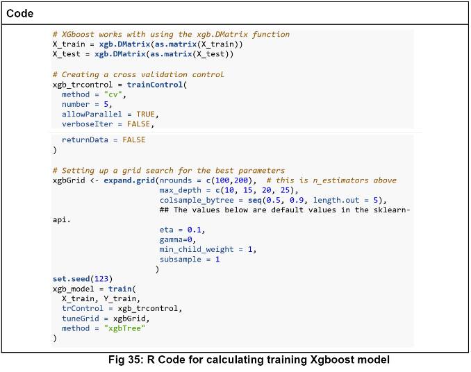
The XgBoost is particularly good at addressing any underfitting or overfitting that may occur when using random-forest or MLR.

Results

The error metrics RMSE and MAPE were used to determine which model performed best on the test set.

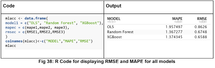
Both random-forest and XgBoost performed relatively well compared with MLR. Ultimately the deciding factor would be computation time. In an ideal scenario both models would be ran and compared side by side as we continued to get results back. The relationship between the observed pH and predicted pH is below.

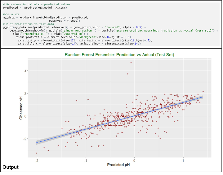
Our model follows the same trends as the actual data follows and visually confirms that random-forest is an appropriate predictor of pH.

Conclusions

While the original data contained 32 predictor variables, only 26 were retained in training models due to multicollinearity, redundancy of information and low-explanation of variability. In an ideal world training multiple models is practical however, from a business and engineering perspective, dimension reduction and model identification is a critical step in the predictive process as choices made can reduce cost associated with acquiring data and training models.

Further conclusions include optimizing manufacturing processes by eliminating elementes that don't contribute to the brand creation. In addition, quality control could be improved; some of these variables presented some readings that could have been from mistakes. Also there maybe possible consilidation opportunities between brands B and C considering how well they coincide with one another.

Special thanks to Layla Quinones, Sergio Ortega, Jack Russo and Neil Shah for teaming up to create an excellently executed final project.

Github Repository